
Site map


Site map |
||
|
|
|
|
| Y2O3 reflection | rel. intensity | measured angular range | time per step |
| (2 1 1) | 11% | 19-22 deg | 4 s |
| (2 2 2) | 100% | 27.5-30.5 deg | 0.5 s |
| (4 0 0) | 25% | 32-35 deg | 2 s |
| (4 4 0) | 44% | 47.5-49.5 deg | 1 s |
| (6 2 2) | 30% | 56.7-58.8 deg | 1.5 s |
| (6 5 1)/(7 3 2) | 2.2% | 67.5-70.3 deg | 20 s |
| (8 4 0) | 5.3% | 80.2-81.7 deg | 10 s |
| (8 7 1)/(8 5 5)/(7 7 4) | 2.9% | 100.5-102.3 deg | 20 s |
| (10 4 4)/(8 8 2) | 1.5% | 111.4-113.8 deg | 40 s |
For extracting the geometric part from the measured standard profiles, a high accuracy of the standard measurement must be achieved. Grain statistic errors should be minimised by appropriate sample preparation and sample illumination. Sufficient counting statistic can be achieved by large counting intervals. Many long-term intensity fluctuations restrict the accuracy capable by a single scan. Therefore, we have added all the nine partial ranges into a 6 hour scan, which was measured 20 times. This method was chosen to test the extracting procedure using different data quality by different scan counts. The reference measurements was done for a Siemens D 5000 device, with a Cu long fine focus tube, Ni filter, primary beam Goebel mirror without Soller collimator, 0.2 mm receiving slit and a scintillation detector. This configuration cannot be described by our raytracing FPA method.
y2o3lprof.par result
file of the Rietveld refinement mentioned on the site
Standard Specimen. We delete the most of the
lines. In following, we must unify some multiplet lines which VERZERR is unable
to handle. For example the four lines
4   1.991656E-02  7.4245083 0.00056098 0.00000031470 ... 7 3 2
4   3.284202E-03  7.4245083 0.00056098 0.00000031470 ... 7 2 3
4   1.191584E+00  7.4245083 0.00056098 0.00000031470 ... 6 5 1
4   1.309926E+00  7.4245083 0.00056098 0.00000031470 ... 6 1 5
must be unified to one:
4 2.524711E+00 7.4245083 0.00056098 0.00000031470 ... 732 ... 723 ... 651 ... 615This is done by adding the intensities (second column) and buiding weighted averages of B1 (fourth column) and B2 (fifth column). In this case no averaging is needed, the fourth and fifth columns do contain identic values between all the multiplet lines. As a final action, set the header entry
PEAKZAHL (german for line count) to the
remaining count of lines. In following, only the heading line plus the
nine selected reference lines remain:
PEAKZAHL=9 TITEL=y2o3t3d1502 LAMBDA=CU ...
4   9.464530E+00  2.3096569 0.00056098 0.00000031470 ... 2 1 1
4   8.971993E+01  3.2663482 0.00056098 0.00000031470 ... 2 2 2
4   2.296439E+01  3.7716540 0.00056098 0.00000031470 ... 4 0 0
4   4.405558E+01  5.3339242 0.00056098 0.00000031470 ... 4 4 0
4   3.174841E+01  6.2545805 0.00056098 0.00000031470 ... 6 2 2
4   2.524711E+00  7.4245083 0.00056098 0.00000031470 ... 7 3 2 ... 7 2 3 ... 6 5 1 ... 6 1 5
4   6.138161E+00  8.4336747 0.00056098 0.00000031470 ... 8 4 0 ... 8 0 4
4   2.615395E+00 10.0675612 0.00056098 0.00000031470 ... 8 7 1 ... 8 5 5 ... 8 1 7 ... 7 7 4
4   1.062661E+00 10.8332513 0.00056098 0.00000031470 ... 10 4 4 ... 8 8 2
y2o3lprof19.sav file as follows:
STANDARDPAR=y2o3lprof
VAL[1]=val\y2o3a2.raw
VAL[2]=val\y2o3a3.raw
VAL[3]=val\y2o3a4.raw
VAL[4]=val\y2o3a5.raw
VAL[5]=val\y2o3a6.raw
VAL[6]=val\y2o3a7.raw
VAL[7]=val\y2o3a8.raw
VAL[8]=val\y2o3a9.raw
VAL[9]=val\y2o3a10.raw
VAL[10]=val\y2o3a11.raw
VAL[11]=val\y2o3a12.raw
VAL[12]=val\y2o3a13.raw
VAL[13]=val\y2o3a14.raw
VAL[14]=val\y2o3a15.raw
VAL[15]=val\y2o3a16.raw
VAL[16]=val\y2o3a17.raw
VAL[17]=val\y2o3a18.raw
VAL[18]=val\y2o3a19.raw
VAL[19]=val\y2o3a20.raw
VERZERR=y2o3lprof
pi=2*acos(0)
POL=sqr(cos(26.6*pi/180))
WMIN=20.6
WMAX=113
WSTEP=3*sin(pi*zweiTheta/180)
We have excluded the first scan. This scan shows some very poor grain statistics.
Now we start the VERZERR program by selecting
Run→Verzerr
browsing to the y2o3lprof.sav file and open it.
In following, we must interpolate the nine reference lines
in the file y2o3lprof.ger by
Run→MakeGEQ
Here follow some exemplary plots of the geometric part G of the
line profiles:
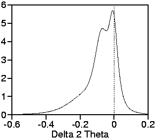
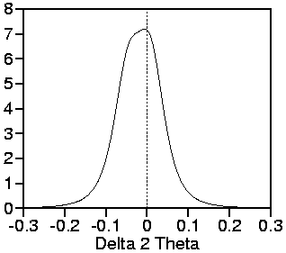
Plots of the learnt geometric
part for the two exemplary angles
25° and 90°.
These learnt geometric profile parts are less acurate than those simulated by raytracing. The main reason: Learnt profiles require an extraction procedure which gives deconvolution oscillations. Raytracing simulates the geometric part itself.
However, the asymmetry of the flanks is more critical than the sharp oscillations which will be predominated by the spectral part of the profile. Therefore, no significant differences in Rietveld refinement are visible.